Troubleshooting the Scheduling Algorithm

This page is dedicated to troubleshooting the Feature Based Scheduler (FBS) algorithm, which is the main scheduling algorithm for the Scheduler CSC.

In general, this will be the last line of resource users will have to resort to when debuging issues at night time. Nevertheless, one may be interested in inspecting the state of the FBS at any time if they are interested in having a better idea of the scheduler operational conditions.

Before proceding make sure you read and understand the Overview section, which gives a high level description of the Scheduler CSC architecture, the scheduling algorithm and the FBS.

Environment Setup

In short, troubleshooting the FBS boils down to inspecting snapshots of the Python object that represents a survey configuration. These snapshot are python pickle files generated by the Scheduler CSC that can be loaded on different machines, so long as the environment used to load them is compatible with that of the machine that generated it.

Unfortunately, the standard nublado environment has a different set of packages than the Scheduler CSC. Therefore we need to create a new environment on nublado to be able to load and inspect the snapshots generated by the Scheduler.

The process is as follows:

1. From your nublado instance, open a new terminal and load the DM environment with:

   source $LOADSTACK
   

2. Create a new conda environment:

   conda create --name scheduler-dev python=3.8
   

3. Activate the new environment:

   conda activate scheduler-dev
   

4. Install the rubin-sim package with mamba:

   mamba install -c lsstts -c conda-forge rubin-sim ipykernel
   

   The rubin-sim package contains several modules for simulating and analysing Rubin data, and includes the feature based scheduler module, we will need to inspect the snapshots.

5. Create a notebook environment with the scheduler-dev conda environment:

   ipython kernel install --name "scheduler-dev" --user
   

   This will allow us to select the “scheduler-dev” environment for our Jupyter notebooks.

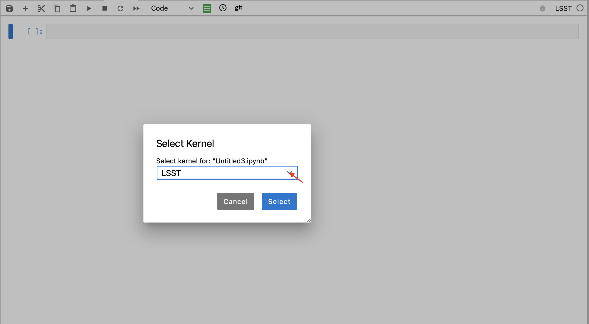
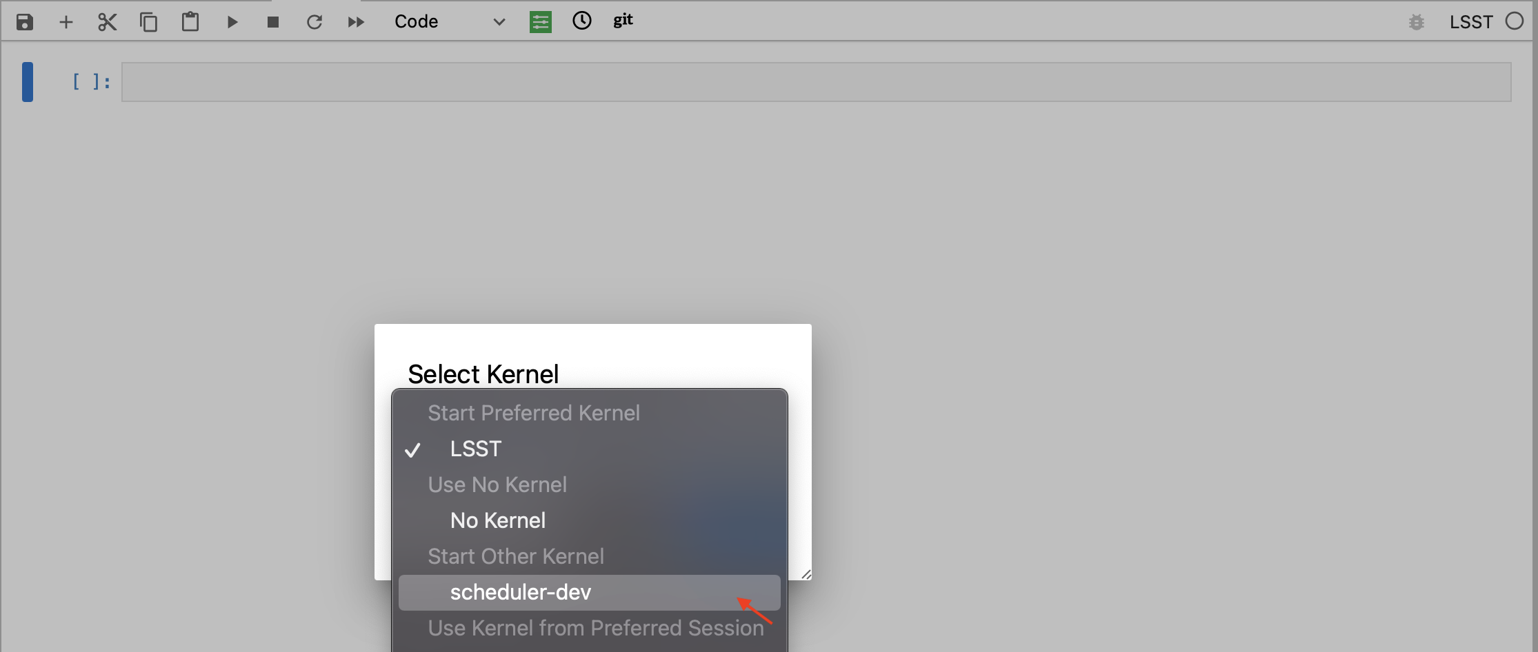
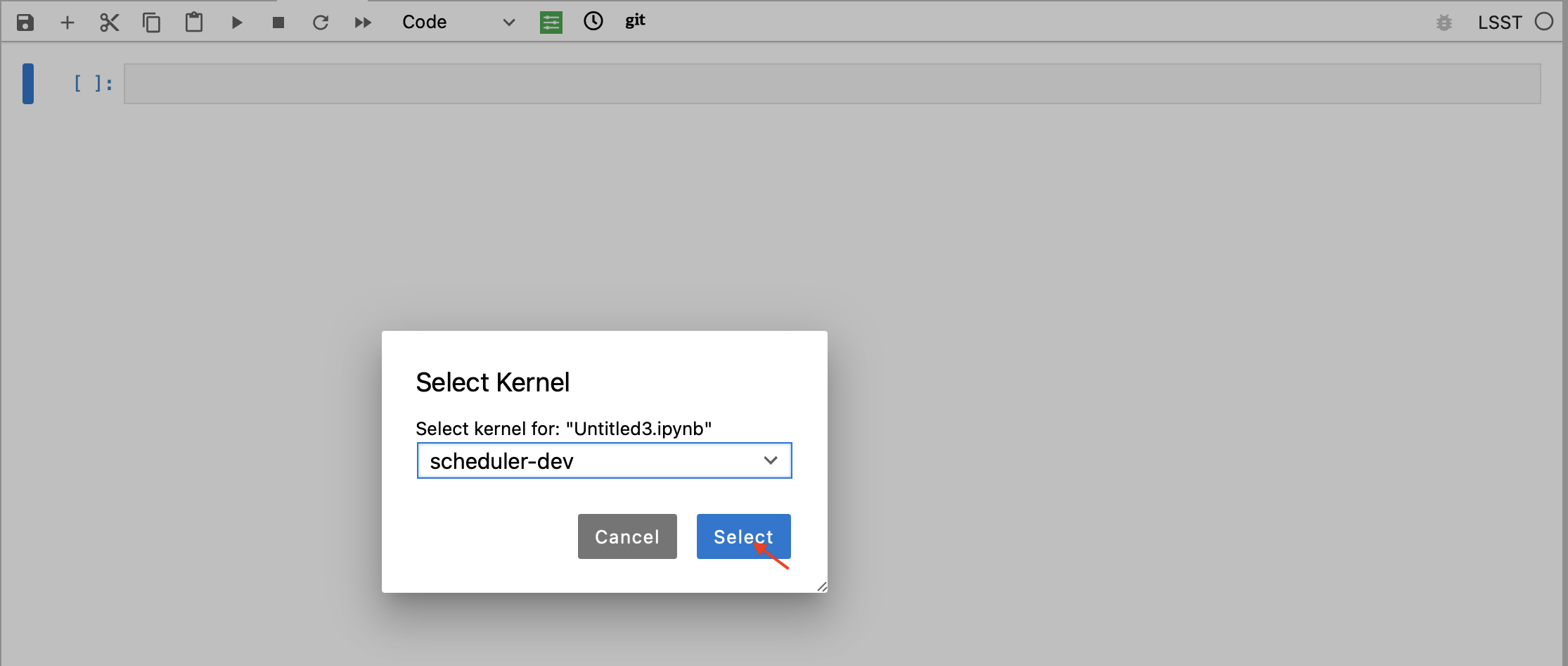
After the steps above are completed, create a new notebook. On the top-right-hand side, click on the environment name, where it is says “LSST” and follow the sequence below to select the “scheduler-dev” environment.

You are now ready to analyse some Scheduler snapshots.

Note

The environment we created to analyse the scheduler snapshots does not have the libraries required to access the control system. Keep that in mind for the following procedures.

Retrieving Snapshots

To retrieve a snapshot created by Scheduler, first we need to find its url. For that, follow the Find Last Scheduler Snapshot procedure.

Once you have the url you can retrieve the snapshot directly from a notebook.

We will use this same notebook to analyse the data, so we start by loading all the libraries we will need.

import io
import os
import math
import pickle
import importlib

import urllib.request

import numpy as np
import healpy as hp

In the cell below we use the same url found in Find Last Scheduler Snapshot, make sure to update the entire string with the appropriate value.

uri = "https://s3.cp.lsst.org/rubinobs-lfa-cp/Scheduler:2/Scheduler:2/2022/02/17/Scheduler:2_Scheduler:2_2022-02-18T09:26:04.347.p"

Now we use urlretrieve to download the file and save it to a local file named scheduler_snapshot.p.

dest, _ = urllib.request.urlretrieve(url=uri, filename="./scheduler_snapshot.p")

Finally, we load the content of the snapshot.

with open(dest, "rb") as fp:
    scheduler, conditions = pickle.load(fp)

As you can see from the code above, the snapshot contains two different objects when unpacked; scheduler and conditions. The first object, as the na suggests, contains the FBS snapshot. The second object contains a snapshot of the last set of telemetry passed to the scheduler. We will need these two objects for the exploratory analysis we will do next.

The conditions Snapshot

Before diving into the scheduler snapshot, let us take a quick glance at the conditions snapshot.

As mentioned above this object contains a snapshot of the telemetry stream. You can check what are all the attributes on this object with the following:

[attr for attr in dir(conditions) if not attr.startswith("__")]

You will notice it contains things like telAlt, telAz, rotTelPos, telDec, telRA, which are determined from the observatory state. There are things like wind_direction and wind_speed which are obtained from the weather station telemetry stream. These are all single scalars.

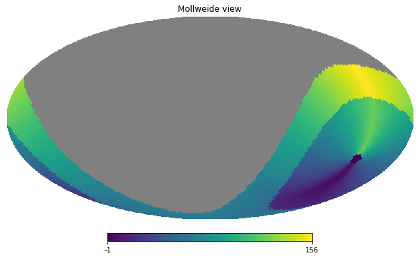
Nevertheless, the telemetry stream also contains some healpix maps. Probably the most interesting one is slewtime, which contains a map of the slew time constructed by the observatory model. We can visualize the slew time healpix map with the following:

hp.mollview(conditions.slewtime)

Analysing the scheduler Snapshot

The first step in analysing the scheduler snapshot is understanding its structure. As mentioned in Overview and shown in the FBS architecture diagram, there is an hierarchical tree of surveys, basis functions and features.

On the scheduler snapshot that can be seen by the following:

scheduler.survey_lists

The survey_lists attribute of the scheduler object contains a list of lists of Survey objects. Each Survey object contains a basis_functions which is a list of BasisFunction objects. Inspecting the features are usually less useful, but each BasisFunction object contains a survey_features attribute which is a dictionary of features.

The following code snippet can produce a textual overview of the structure of the scheduler:

display_filename_prefix_middle = '├──'
display_filename_prefix_last = '└──'
display_parent_prefix_middle = '    '
display_parent_prefix_last = '│   '

def get_classname(obj):
    return f"{obj!r}".split(" ")[0].split(".")[-1]

def generate_prefix(current_prefix, list_size):
    prefix = current_prefix
    if i < list_size-1:
        prefix += display_filename_prefix_middle
    else:
        prefix += display_filename_prefix_last
    return prefix

survey_size = ", ".join([f"{len(survey)}" for survey in scheduler.survey_lists])
print(f"Total number of surveys: {sum([len(survey) for survey in scheduler.survey_lists])} -> [{survey_size}]")

print(f"Number of survey lists: {len(scheduler.survey_lists)}")
for i, survey_list in enumerate(scheduler.survey_lists):
    prefix = generate_prefix(display_parent_prefix_middle, len(scheduler.survey_lists))
    print(f"{prefix} Number of surveys in list {i+1}: {len(survey_list)}")

    for j, survey in enumerate(survey_list):
        pprefix = generate_prefix(display_parent_prefix_middle + display_parent_prefix_last + display_parent_prefix_middle, len(survey_list))
        print(f"{pprefix} {get_classname(survey)}[{survey.survey_name}]")

        for k, basis_function in enumerate(survey.basis_functions):
            ppprefix = generate_prefix(display_parent_prefix_middle + display_parent_prefix_last + display_parent_prefix_middle + display_parent_prefix_last, len(survey.basis_functions))
            is_healpix = "[helpix map]" if hasattr(basis_function(conditions), '__len__') else ""
            print(f"{ppprefix} {get_classname(basis_function)} :: Feasibility: {basis_function.check_feasibility(conditions)} {is_healpix}")

The code above will show something like the following:

Total number of surveys: 236 -> [1, 212, 11, 12]
Number of survey lists: 4
    ├── Number of surveys in list 1: 1
    │       └── Greedy_survey[cwfs]
    │       │   ├── Not_twilight_basis_function :: Feasibility: True
    │       │   ├── Slewtime_basis_function :: Feasibility: True [helpix map]
    │       │   ├── Slewtime_basis_function :: Feasibility: True
    │       │   ├── Slewtime_basis_function :: Feasibility: True
    │       │   ├── Moon_avoidance_basis_function :: Feasibility: True [helpix map]
    │       │   ├── Zenith_shadow_mask_basis_function :: Feasibility: True [helpix map]
    │       │   ├── VisitGap :: Feasibility: False
    ├── Number of surveys in list 2: 212
    │       ├── FieldSurvey[LATISS_MD02_00000001]
    │       │   ├── Not_twilight_basis_function :: Feasibility: True
    │       │   ├── Hour_Angle_limit_basis_function :: Feasibility: False
    │       │   ├── Slewtime_basis_function :: Feasibility: True [helpix map]
    │       │   ├── Slewtime_basis_function :: Feasibility: True
    │       │   ├── Slewtime_basis_function :: Feasibility: True
    │       │   ├── Moon_avoidance_basis_function :: Feasibility: True [helpix map]
    │       │   ├── Zenith_shadow_mask_basis_function :: Feasibility: True [helpix map]
    │       │   ├── VisitGap :: Feasibility: False
    │       │   ├── AvoidDirectWind :: Feasibility: True [helpix map]
    │       │   ├── BalanceVisits :: Feasibility: True
    │       ├── FieldSurvey[LATISS_MD02_00000002]
    │       │   ├── Not_twilight_basis_function :: Feasibility: True
    │       │   ├── Hour_Angle_limit_basis_function :: Feasibility: False
    │       │   ├── Slewtime_basis_function :: Feasibility: True [helpix map]
    │       │   ├── Slewtime_basis_function :: Feasibility: True
    │       │   ├── Slewtime_basis_function :: Feasibility: True
    │       │   ├── Moon_avoidance_basis_function :: Feasibility: True [helpix map]
    │       │   ├── Zenith_shadow_mask_basis_function :: Feasibility: True [helpix map]
    │       │   ├── VisitGap :: Feasibility: False
    │       │   ├── AvoidDirectWind :: Feasibility: True [helpix map]
    │       │   ├── BalanceVisits :: Feasibility: True
    ...

This allows you to see which surveys are defined, which basis functions are part of each survey, the “feasibility” of each basis function and a note when the basis function is a helpix map (this will be useful furthermore). Feasibility, is the “first line of defence” of a basis function. It determines whether a basis function yield observations for a given set of conditions. This “superseeds” the actual “score” of the basis function.

In the case above you can see, for instance, that both the Hour_Angle_limit_basis_function and VisitGap on the FieldSurvey[LATISS_MD02_00000001] survey are False. If one basis function from a survey is not feasible, it means it cannot be scheduled at this time. It this case, the Hour_Angle_limit_basis_function is telling us the survey is out of the specified hour angle limits, and therefore cannot be observed. Furthermore, the VisitGap basis function specifies a minimum time between consecutive observations of a survey have not passed.

Usually, when trying to understand lack of observations, the first thing to check is whether there are feasible surveys in the first place and, if not, why they are not feasible. In most cases, it is obvious from the basis function name.

It may still happen that although all basis functions are feasible, we still do not get targets. This happens mostly because “feasibility” is a high level check, and details on the basis functions may still render the survey non-observable, although still feasible. To get to this level of understanding, one needs to analyse the basis function value. Some knowledge of the different kinds of surveys might also be necessary to get a full picture.

In the summary above, there are two different types of surveys; Greedy_survey and FieldSurvey. The Greedy_survey is a “region” based survey, which allows users to specify an area on the sky to be surveyed according to several constraints imposed by the basis functions. The FieldSurvey, allows one to specify a field (determined by its RA and Dec coordinates), which will be observed according to the constraints imposed by its basis functions.

Note

Although the imaging survey on AuxTel is supposed to map a “region” of the sky, it would require an extremely high sky resolution to allow us to define it in terms of a Greedy_survey. Therefore we use FieldSurvey configured with individial pointings. This allows us to run the scheduler with a lower resolution and still map the region.

In the example above we already know that the LATISS_MD02_* fields are still outside the hour angle limit, so they won’t be observable. Still let us explore some of the basis functions rewards as an exercice.

The first thing to keep in mind is that basis functions reward values can either be single floats, or healpix maps. The ones we will be most interested in analysing are healpix maps, probably comparing them with the current position of the telescope and, in the case of FieldSurvey-like surveys, the position of the field.

Let’s analyse the basis function of FieldSurvey[LATISS_MD02_00000001], the first survey on the second list of surveys. We start by extracting the survey into a variable:

survey = scheduler.survey_lists[1][0]

In the summary above we show a note when the basis function returns a healpix map. For FieldSurvey[LATISS_MD02_00000001] we can see that there are four basis functions in this condition; Slewtime_basis_function, Moon_avoidance_basis_function, Zenith_shadow_mask_basis_function and AvoidDirectWind. We can show each of these maps with the current position of the telescope and the position of the field with the following:

fig_num = 1
for bfs in survey.basis_functions:
    bfs_value = bfs(conditions)
    if hasattr(bfs_value, "__len__"):
        hp.mollview(bfs_value, title=get_classname(bfs), fig=fig_num)
        hp.projscatter(np.degrees(survey.ra), np.degrees(survey.dec), lonlat=True, coord="E", color="red")
        hp.projscatter(np.degrees(conditions.telDec), np.degrees(conditions.telDec), lonlat=True, coord="E", color="green")
        fig_num += 1

The position of the field is shown as a red dot in the map, and the position of the telescope as a green dot. In this particular case, the telescope was pointing towards the south celestial pole. Hence the green dot is shown as the bottom part of the sky projection.

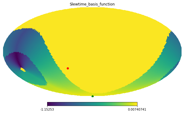
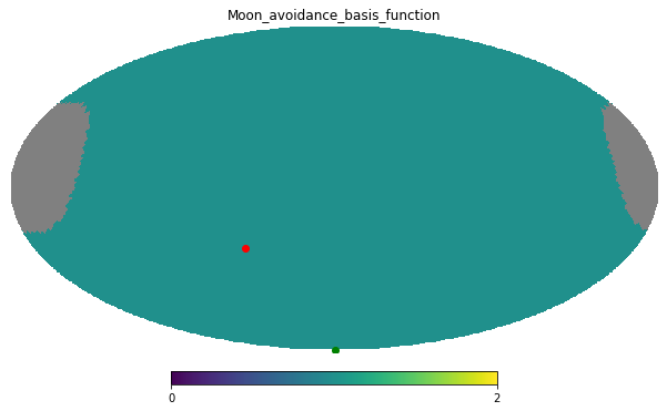
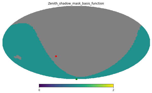
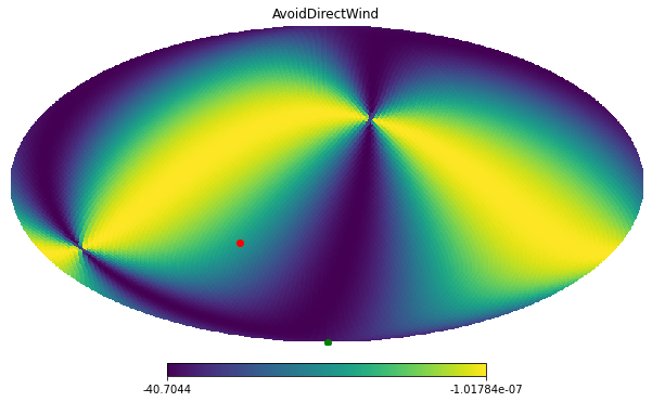
From the images above one can see why the hour angle limit is yielding the survey unfeasible, as the targets are still below the horizon, as can be seen on the Slewtime_basis_function and the Zenith_shadow_mask_basis_function.

This should give you enough information to allow you to throubleshoot most conditions experienced by the scheduler and also to understand what the scheduler is doing at a particular moment in time.